Copulas

A high-level introduction to modelling dependence

Why copulas?

Many questions across disciplines involve several variables at once: stock indices from two or more companies, rainfall and river discharge, temperature at neighbouring stations, deforestation this year and last year. How these variables behave together matters as much as how each behaves on its own. A flood risk assessment, for example, depends on how likely high discharge and high water levels are to occur at the same time.

Copulas are a tool for exactly this. They separate a multivariate distribution into two parts that can be studied and modelled independently:

• the margins, i.e. the distribution of each variable on its own, and
• the copula, i.e. the dependence structure that links them.

This separation makes it possible to combine any kind of marginal distribution (skewed, heavy-tailed, bounded) with a dependence structure that goes far beyond a single correlation coefficient.

Margins and joint distributions

Think of the body weight and body height of students. Each of the two has its own distribution, its margin. Taken together, the pairs (weight, height) follow a joint distribution, which in a scatterplot shows up as a cloud of points with some positive dependence.

A joint distribution is fully described by its joint cumulative distribution function (cdf)

\[ H(x, y) = P(X \le x,\ Y \le y), \]

the probability of observing a pair in the lower-left quadrant of the point \((x, y)\). The margins \(F(x) = P(X \le x)\) and \(G(y) = P(Y \le y)\) are the views of this distribution from each axis.

A simple but central fact makes copulas work: if a continuous random variable \(X\) has the cdf \(F\), then \(F(X)\) is uniformly distributed on \([0, 1]\). Transforming every variable through its own cdf therefore puts all variables on the same scale, no matter how differently they were distributed before.

Sklar’s theorem

Sklar’s theorem (1959) states that every joint distribution can be written as

\[ H(x, y) = C\big(F(x),\, G(y)\big), \]

where \(C\) is a copula: a joint distribution function on the unit square \([0, 1]^2\) whose margins are uniform. If the margins \(F\) and \(G\) are continuous, the copula \(C\) is unique.

Read the other way round, the theorem is a construction kit: pick any margins, pick any copula, and their combination is a valid joint distribution. The same holds in more than two dimensions.

Measuring dependence

The most familiar measure of dependence is Pearson’s correlation coefficient. It describes linear dependence and is affected by the shape of the margins. Rank-based measures avoid this by only comparing the order of observations:

• Spearman’s rho is Pearson’s correlation computed on the ranks of the data.
• Kendall’s tau compares all pairs of observations and counts how many are concordant (both variables increase together) versus discordant.

The figure below shows one and the same dependence structure combined with two different sets of margins. Pearson’s correlation changes with the margins, while Kendall’s tau stays the same. After a rank transformation \(u = \operatorname{rank}(x) / (n + 1)\), both samples become identical: what remains is the copula.

The same dependence with normal and log-normal margins. Only rank-based measures and the rank-transformed sample are unaffected by the margins.

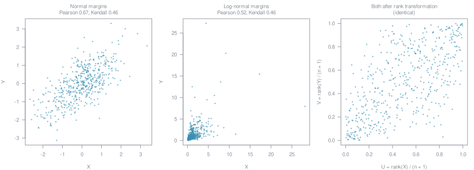
For many copula families, Kendall’s tau and Spearman’s rho are in a one-to-one relation with the copula parameter. This offers a simple way to estimate a copula from data.

Copula families

There are many parametric copula families, and they differ most in their tails: how strongly the variables depend on each other when both take extreme values. The four samples below all have the same Kendall’s tau of 0.5, yet their dependence structures are clearly different:

Samples of 500 points from four copula families, all with Kendall’s tau of 0.5.

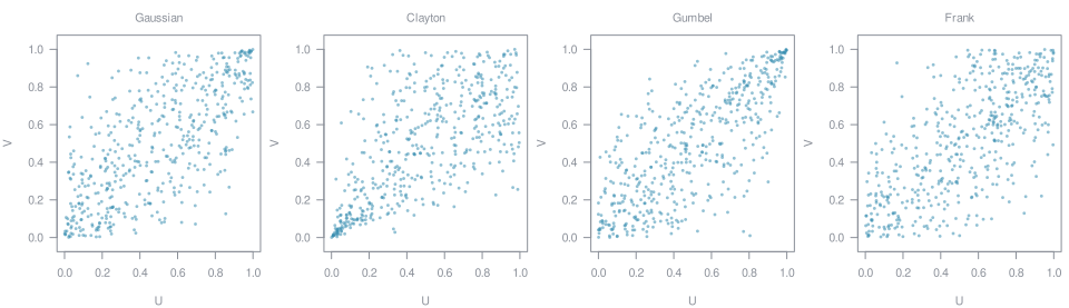
• The Gaussian copula is symmetric and has no tail dependence: joint extremes are comparatively rare.
• The Clayton copula shows strong dependence in the lower tail: small values tend to occur together.
• The Gumbel copula shows strong dependence in the upper tail: large values tend to occur together, a typical pattern for floods or heat waves.
• The Frank copula is symmetric and, like the Gaussian, has no tail dependence; joint extremes are even rarer.

Beyond these classical families, asymmetric copulas allow for dependence structures that are not mirror-symmetric. For more than two variables, vine copulas build a high-dimensional copula from a cascade of bivariate building blocks, which keeps the model flexible and tractable.

Tails matter. Heavy-tailed distributions assign far more probability to extreme values than the normal distribution: a value four standard deviations above the mean is about 100 times more likely to be exceeded under a Gumbel distribution than under a normal distribution with the same mean and variance, and five standard deviations above the mean, more than 3,000 times. A dependence model that ignores the tails can severely underestimate the risk of joint extremes.

Modelling with copulas

A typical copula analysis follows a few steps:

1. Fit the margins. Each variable is modelled on its own, for example by maximum likelihood. This is a one-dimensional task and well established in statistics.
2. Transform to the unit square. Either through the fitted margins or, without any assumption, through the rank transformation.
3. Explore the dependence. Scatterplots and density plots of the rank-transformed data reveal tail behaviour and asymmetries that a correlation coefficient hides.
4. Fit a copula. Choose a family and estimate its parameters, by inverting Kendall’s tau or by maximum likelihood.
5. Check the fit. Goodness-of-fit tests compare the fitted model with the data, often by parametric bootstrap.
6. Use the model. Combine copula and margins to compute joint probabilities, conditional distributions, return periods or risk maps, and to simulate new data.

Real data does not always meet the assumptions of continuous margins. Rainfall, radiation measurements or deforestation often contain a large share of zeros. For such zero-inflated data, the unit square can be split into a part for the zeros and a part for the positive values, each modelled separately. In a study on deforestation in the Brazilian Amazon, this approach was used to derive maps of the risk that deforestation exceeds a given threshold (Gräler et al. 2010, see publications).

Getting started in R

The copula package provides a wide range of copula families together with estimation, simulation and goodness-of-fit tools. VineCopula adds bivariate families and vine copulas.

library(copula)

# simulate from a Gumbel copula with Kendall's tau of 0.5
cop <- gumbelCopula(iTau(gumbelCopula(), 0.5))
u <- rCopula(500, cop)

# rank-transform data and estimate the copula parameter
fit <- fitCopula(gumbelCopula(), pobs(u), method = "itau")
summary(fit)

The copulatheque lets you explore different copula families interactively in the browser.

Multivariate return periods

In hydrology, design values are usually expressed as return periods: a 100-year flood is one that is exceeded on average once in 100 years. For a single variable with cdf \(F\) and an average time \(\mu\) between events (one year for annual maxima), the return period of a value \(x\) is

\[ T(x) = \frac{\mu}{1 - F(x)}. \]

A flood, however, is characterised by more than one variable. Dams and retention basins have to cope with both the peak discharge and the flood volume, and the two are strongly dependent. For two or more variables there is no single definition of “exceeding” a design event, and different definitions lead to quite different design values. With \(u = F(x)\), \(v = G(y)\) and the copula \(C\), three common definitions are:

• OR: an event is critical if either variable exceeds its design value, \(T_{\text{OR}} = \mu \,/\, \big(1 - C(u, v)\big)\).
• AND: an event is critical only if both variables exceed their design values, \(T_{\text{AND}} = \mu \,/\, \big(1 - u - v + C(u, v)\big)\).
• Kendall: an event is critical if it is more extreme in terms of the copula, i.e. if \(C(U, V) > t\). With the Kendall distribution function \(K_C(t) = P\big(C(U, V) \le t\big)\), this gives \(T_{\text{KEN}} = \mu \,/\, \big(1 - K_C(t)\big)\).

The figure shows the difference for the flood peaks and volumes of 494 simulated flood events, the data set of the multivariate return period demo in sfcopula. Peak and volume are strongly dependent (Kendall’s tau 0.85), and a Clayton copula describes their dependence well. Each line marks all combinations of peak and volume that have a return period of exactly 10 years under one of the definitions:

Critical lines of the 10-year return period under the OR, AND and Kendall definitions for flood peak discharge and volume, shown on the copula scale. Points are simulated flood events.

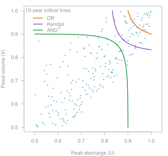
All three lines claim to describe a 10-year event, but they are far apart. Assuming one flood per year, a 10-year event should be exceeded by about one in ten floods. In the sample, 10.9 % of the events lie beyond the Kendall line, close to the intended 10 %. Only 4.7 % lie beyond the OR line, so in terms of Kendall’s definition the OR line actually corresponds to a return period of about 23 years. Beyond the AND line lie 15.2 % of the events, so it describes a more frequent event than intended.

Which definition is appropriate depends on what makes an event dangerous for the structure at hand. The review by Gräler et al. (2013, see publications) compares these and further definitions and their consequences for synthetic design hydrographs. The sfcopula package provides the Kendall distribution function and the related return periods:

library(sfcopula)

# flood peak and volume of 494 simulated flood events
data("simulatedTriples")
peakVol <- rank_transform(triples[, 1], triples[, 3])

# fit a Clayton copula by maximum likelihood
copQV <- fitCopula(claytonCopula(), as.matrix(peakVol), method = "ml")@copula

# Kendall distribution function K(t) = P(C(U, V) <= t)
kendallFunQV <- get_kendall_distr(copQV)

# critical level of the 10-year Kendall return period (one event per year)
critical_level(kendallFunQV, 10, mu = 1)                     # 0.833

# Kendall return period of the 10-year OR critical level
kendall_rp(kendallFunQV, cl = 0.9, mu = 1, copula = copQV)   # 23.3 years

Spatial copulas